The activities performed by DISIT Lab within the AMMIRARE project focused on defining data models, developing acquisition (ingestion) pipelines, and designing and implementing interactive interfaces in the form of multi-data dashboards integrated into the Snap4City platform (https://www.snap4city.org/).
These dashboards serve both as an interface for entering data into Snap4City and for visualizing and inspecting those data. In this way, the platform implements both an archiving system (in which data are semantically enriched) and a decision-support tool that enables operators to analyze the data to monitor the coastal environment.
All dashboards and tools are implemented following a multi-user paradigm with strict rules on data ownership and delegation. The system is designed to allow each project partner to have three types of user accounts: operator and viewer.
- Operator supervises data loading into the platform and is the owner of the uploaded data.
- Demo has read-only permissions and a limited permission to upload data.
- Viewer is granted read-only permissions to access all data uploaded by any project partner.
More specifically, DISIT Lab developed the following tools for data acquisition and visualization.
2.1 Data search
To provide a single access point to all dashboards/tools, a Data Search dashboard was created that acts as the main menu and provides functions for searching available data and displays links to access the tools used for data visualization (see figure 1). Each dashboard also includes a button to return to the main menu.
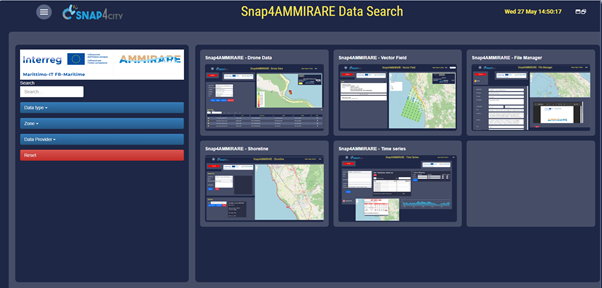
figure 1: Dashboard Data Search (main menu)
The side menu allows you to filter dashboards by name (using the search text box) or via side filters.
The Data Search dashboard is accessible to authorized users at the following link: https://www.snap4city.org/dashboardSmartCity/view/Gea-Night.php?iddasboard=NDkyOQ==
viewer version
https://www.snap4city.org/dashboardSmartCity/view/Gea-Night.php?iddasboard=NTAxNg==
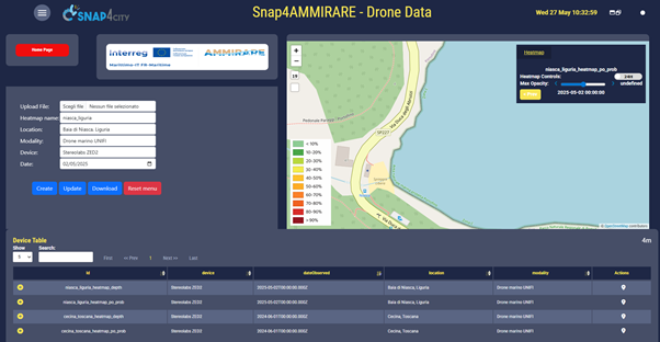
figure 2: Dashboard Drone Data
This dashboard allows users to upload, with versioning, and visualize georeferenced data on a 2D grid, generally acquired through drone scans. The dashboard, shown in the screenshot in figure 2, consists of a panel in the upper left that can be used to upload or update data while also providing a set of descriptive metadata related to the uploaded data. The acquired data will then be managed in the platform by creating a specific semantic entity (according to a specific data model) and associating it with a heatmap calculated on the basis of the provided data values. At the bottom, a table enables searching for inserted data and reloading them for visualization.
In the upper right, a MultiData Map widget enables the visualization of the data, represented as heatmaps and associated with a colormap that represents the data values on a color scale. In the case of subsequent uploads to the same entity, for example to record acquisitions of the same type at later times, the interface provides a time navigation system accessible through the panel in the upper right included in the map, managed with the Next/Prev buttons.
2.2.2 Usage
Data loading is performed from the left menu using the input box "Upload file". The file must necessarily be in .csv format.
Additional metadata is also required to start heatmap creation.
- Heatmap name: This name is used as the basis for identifying the heatmaps generated by the file upload.
A heatmap is identified as [Heatmap name]_heatmap_[csv file column]
For example, using "niasca_liguria" as the heatmap name, it will be possible to identify the heatmaps niasca_liguria_heatmap_depth and niasca_liguria_heatmap_po_prob
- Date: Indicates the day to which the input data refer. In this way, by performing an update, it is possible to give the heatmap a temporal progression.
- Location, Modality and Device describes where and how the data were acquired.
The file is then uploaded and sent to the program on the server, which will process it and create the heatmaps based on the values it contains. This process is asynchronous and is not started immediately after the file is uploaded in order to avoid excessive memory use, especially when large amounts of data need to be uploaded. Therefore, do not worry if the heatmaps are not immediately visible in the table at the bottom of the dashboard.
To view a heatmap on the map, click the corresponding icon in the table. The section with the left menu will also show the previously entered metadata.
The Download button allows you to download the original uploaded file.
The Update button allows the user who created the heatmap to add more data to the heatmap. The date must be changed to start an update, only the operation and the creator user of the heatmaps are allowed to update an existing heatmap.
2.2.3 Input
The dashboard is currently set to create heatmaps concerning depth and the probability of Posidonia oceanica.
The reference model for the input files to be entered in the program is therefore the following.
|
latitude |
longitude |
depth |
po_prob |
|
43.310618432191 |
10.4659683198608 |
4.75 |
0.5 |
|
43.310618432191 |
10.4659744829008 |
4.75 |
0.535841 |
|
43.310618432191 |
10.4659806459408 |
4.75 |
0.535841 |
2.2.4 Notes
Heatmap creation occurs asynchronously with respect to dashboard use; therefore, a few minutes may pass between uploading the input files and creating the dashboards.
A message will be visible in the menu: 'Some uploaded files are still being processed. Heatmap generation is in progress.' if heatmap generation has not yet been completed.
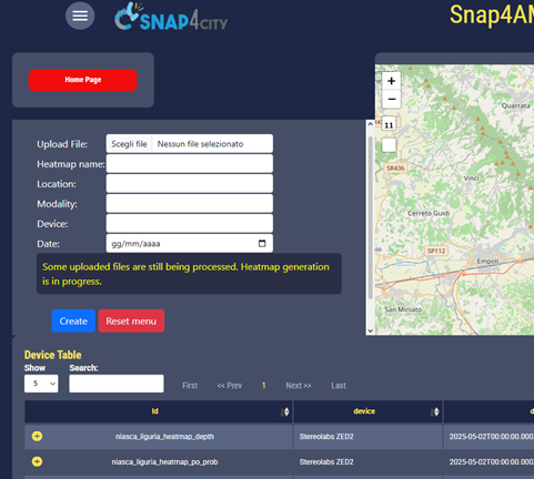
figure 2.1: Dashboard Drone Data
2.2.5 Link
The dashboard is accessible to authorized users at the following link: https://www.snap4city.org/dashboardSmartCity/view/Gea-Night.php?iddasboard=NDkyOA==
Viewer version:
https://www.snap4city.org/dashboardSmartCity/view/Gea-Night.php?iddasboard=NTAwNg==
2.3 Vector field
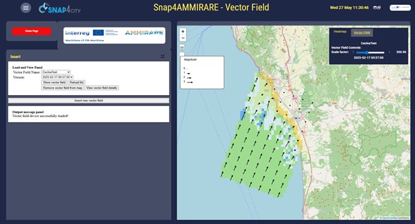
figure 3: Dashboard Vector Field
This dashboard is used to manage georeferenced vector fields that describe natural effects such as waves, winds, etc. It is used to perform three main operations: (i) visualize the inserted vector fields, possibly with the related associated heatmaps, in order to observe and study natural phenomena; (ii) insert new vector fields and possibly create the associated heatmap; (iii) update vector fields by providing new measurements to obtain a temporal evolution of the phenomenon. The dashboard consists of two main parts (see figure 3).
On the left side there is a control panel. From this panel it is possible to load a previously inserted vector field, insert a new vector field and, at the bottom, an area for output messages is included. The uploaded data are automatically processed by the platform and ingested by creating semantic entities, one for the vector field and possibly a second entity for the associated heatmap. Vector fields are indexed in the platform using a specific data model that includes the specifications of the vector field and additional descriptive metadata. Similarly, a specific data model has been defined for the associated heatmaps. On the right side, the MultiDataMap widget is included and is used to show the vector fields.
The vector field is displayed as a series of vectors aligned to a rectangular grid oriented at a defined angle with respect to the North direction. Depending on the map zoom level, a different number of vectors is displayed: as the zoom increases, more vectors appear. Each vector is oriented according to its own direction and has a length proportional to its intensity. Using the slider in the bottom-right panel, it is possible to scale the vector length for better visualization. When multiple versions of the vector field are available, they can be navigated using the Next/Prev buttons in the panel. Moving the mouse over the base point of the vectors displays a popup showing the vector angle and intensity. A legend of vector intensity is shown on the left side of the map. The vector sizes in the legend are updated dynamically based on the selected scale factor.
Under the vector field, a heatmap is shown (if it was created when the vector field was inserted). The heatmap values are encoded according to the colormap shown in the lower-left corner of the map. Using the slider in the Heatmap panel it is possible to change its opacity. Please note that version navigation is controlled only by the vector-field panel. The corresponding heatmaps are loaded automatically.
In the menu on the left side of the dashboard it is possible to load and view an existing vector field, selecting it and its relative version and clicking on “Show vector field”.
After vector field load, it’s also possible to see in detail the features of a vector field by clicking on “View vector field details”.
To create a new vector field, click the Insert new vector field button. A menu will appear with a series of input forms for entering metadata.
Latitude and Longitude indicate the coordinates of the southwestmost point from which the vector field will be created.
Number of rows and Number of columns indicate the distribution of the element on the vectorfield.
ΔX and ΔY indicate the distance between each element row and each column
α angle indicate the general angle of the vector field relative to the north,
Magnitude matrix and Angle matrix representing the values to ingest in the vector field. They can be both inserted directly in the textarea or loaded by a txt file. They are represented by a vector of vectors . (for example see 2.3.4 )
In addition a vector field can be created also a heatmap with the relative colormap.
Following in this paragraph there are some examples of matrices for the vector field. Every vector represents a row, and every value in columns. To be valid, matrices must match the Number of rows and Number of columns values. These examples show a vector field with three rows and ten columns.
Magnitude matrix (meters): [[0,0.5,0.8,1,1.1,1.2,1.3],[1.4,1.5,1.6,1.7,1.8,1.9,2],[2.1,2.2,2.3,2.4,2.5,2.6,3]]
Angle matrix (degree): [[0,15,30,45,60,75,90],[0,-15,-30,-45,-60,-75,-90],[0,5,-5,10,-10,15,-15]]
By convention, values have to be separated by commas and decimal places are indicated by dots.
The dashboard is accessible to authorized users at the following link: https://www.snap4city.org/dashboardSmartCity/view/Gea-Night.php?iddasboard=NDQ1OA==
Viewer version: https://www.snap4city.org/dashboardSmartCity/view/Gea-Night.php?iddasboard=NTAwNw==
2.4 File manager
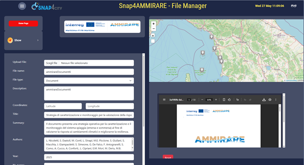
figure 4: Dashboard File manager (Document view)
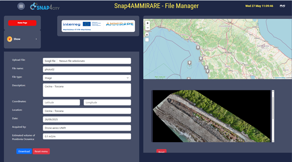
figure 4.1: Dashboard File manager (Orthophoto view)
This dashboard allows the upload of different types of files and their selection through icons displayed on a map.
The dashboard consists of several components: on the left there is a menu for uploading files and entering metadata. At the top right there is a map for selecting the uploaded file and viewing its preview in the bottom-right section.
Specifically, this dashboard is designed for uploading .pdf documents and orthophoto images in .tif format, however its structure is flexible enough to allow the insertion of other types of data with different formats.
Uploaded files are visible on a map via icons, and by clicking on them you can view both the metadata associated with the uploaded file and the document itself, which can be downloaded using a specific button.
The metadata associated depending on the type of file to be uploaded. For example, information such as Authors and Summary is present only for Documents, and other such as Acquired by and Location to Images and Video.
For the file upload to be valid, it is important to enter the coordinates and define the file type. The coordinates are essential for positioning the icon on the map, while the file type is necessary for entering specific metadata.
2.4.3 Input
Accepted formats:
- Images: .jpg, .png, .tiff, .tif
- Video: .mp4, .mov
- Documents: .pdf, .txt, .doc, .docx
The dashboard is accessible to authorized users at the following link: https://www.snap4city.org/dashboardSmartCity/view/Gea-Night.php?iddasboard=NTEyNw==
Viewer version: https://www.snap4city.org/dashboardSmartCity/view/Gea-Night.php?iddasboard=NTEzMA==
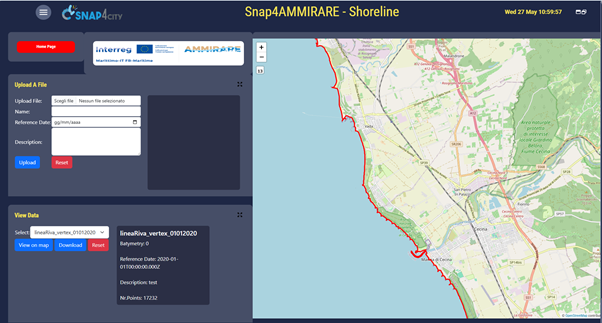
figure 5: Dashboard shoreline
2.5.1 Description
This dashboard allows the creation and visualization of a trajectory representing a shoreline or a bathymetric line to be shown on a map.
The dashboard consists of a menu in the upper left for uploading a CSV file with the list of coordinates and bathymetry (in the case of shorelines, a value of 0) and some metadata to be entered. Once uploaded, in the bottom-left menu it will be possible to select the uploaded shoreline and display it on the map. Some metadata such as the number of trajectory points and the bathymetry value will also be displayed in a space in the bottom left menu.
In the view version of this dashboard, the shoreline upload menu is not present. The user can therefore only view the existing shorelines, without being able to create his own.
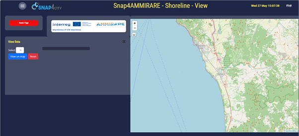
figure 5.1 : Dashboard shoreline (viewer version)
2.5.2 Input
The input file is a CSV file with the following characteristics: a vertex_index, which is used to order the coordinates so that the trajectory is drawn without overlaps or errors. X and Y represent the coordinates and Z represents the shoreline (if it has value 0) or the bathymetry.
|
vertex_index |
X |
Y |
Z |
|
10.5188894028013 |
43.0825372763435 |
-20 |
|
|
1 |
10.5188933858181 |
43.0825409306627 |
-20 |
|
2 |
10.5188992110557 |
43.0825672252318 |
-20 |
2.5.3 Notes
To avoid excessive memory load and excessive loading times, based on the zoom level on the map the points undergo a clustering process whereby the lower the zoom, the greater the clustering. To obtain a higher level of detail, it is advisable to zoom in.
2.5.4 Link
The dashboard is accessible to authorized users at the following link: https://www.snap4city.org/dashboardSmartCity/view/Gea-Night.php?iddasboard=NTEyOA==
Viewer version:
https://www.snap4city.org/dashboardSmartCity/view/Gea-Night.php?iddasboard=NTEzNA==
2.6 Time series
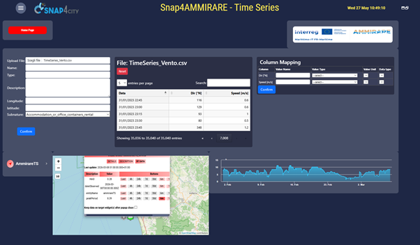
figure 6: Dashboard time series
2.6.1 Description
This dashboard allows the creation of customized time series by uploading CSV files with the data, defining the columns and finally creating a device that represents a temporal sequence. The time series are visible on a map through icons; by clicking the icon and selecting a button related to one of the values in the right section, the time-series chart will show the requested data.
The operation occurs in several steps. In the first, a file with the values that will compose the time series is inserted and the column characteristics of the device you intend to create are defined. Once these characteristics are defined, a corresponding device will be created with the corresponding values.
The timeseries cannot be created directly when the file is uploaded because it must first be verified for accuracy (for example, whether a field contains the correct date and time) and because, in this case, there is no pre-existing device model, so its characteristics and columns must be defined before proceeding. The advantage of this approach is that it is possible to create very different timeseries, which can represent many different types of data with their appropriate metrics.
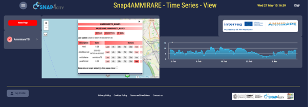
figure 6.1: Dashboard time series (viewer version)
2.6.2 Usage
In the left menu select upload file and upload a CSV file. Enter the following metadata.
Name indicates the name of the time series: the time series are identified by the prefix AmmirareTS followed by the name entered in the menu. For example, choosing the name "waves" AmmirareTS_waves. (The name cannot contain spaces or non-alphanumeric characters)
Longitude and Latitude are necessary for visualization on the map.
Type can refer to the type of data (Temperature, Waves, Wind, Precipitation, etc.) in the Time Series.
To display the time series, click an icon on the map; a popup will appear with the metadata (showing the most recent by default) and buttons with the time intervals to show, which can range from the last 4 hours up to 10 years (Latest, 4h, 24h, 7d, 30d, 6m, 1y, 2y, 10y). Click a button to display the data for this period in the chart, related to a specific metric.
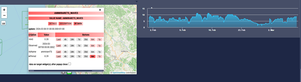
figure 6.2: Widget map and time series
The column name in the device cannot be extracted directly from the CSV file because there may be invalid characters or spaces that the program does not accept.
Once the file upload has been started with the Confirm button, two new sections will be shown in the dashboard: a table with a view of the data contained in the CSV file and a table for column mapping.
To be valid, a file to be uploaded must contain a list of valid dates, and the columns must be mapped by assigning each of them a Value name (which represents the name that the column will have in the final device), a Value type, a Value Unit and a Data Type. This operation is used to define the type of data represented by the column and describe it according to the schema used by Snap4City.
Once finished, click the "confirm" button below the column mapping table.
2.6.3 Input
The files to be uploaded must necessarily be in CSV format and have a column named Data or Date with the dates and times of the time series. The following columns may vary from file to file.
Unlike the other dashboards, CSV files can have a highly variable number of columns and content.
|
Data |
Hm0 |
Tp |
|
01/02/2026 00:00 |
0.44 |
7.62 |
|
01/02/2026 01:00 |
0.43 |
7.62 |
|
01/02/2026 02:00 |
0.44 |
7.63 |
Data loading into the time series takes place asynchronously with respect to device creation in order to avoid excessive load when running the program. For this reason, initially, when selecting a time series in the first few minutes, the temporal sequence may not yet be complete.
The dashboard is accessible to authorized users at the following link: https://www.snap4city.org/dashboardSmartCity/view/Gea-Night.php?iddasboard=NTA1Ng==
Viewer version: https://www.snap4city.org/dashboardSmartCity/view/Gea-Night.php?iddasboard=NTA1Nw==
-- end ---
