
https://www.snap4city.org/dashboardSmartCity/view/index.php?iddasboard=MzA4NA==
In many applications, the access of the tpyical time trends of certain variable is very useful. The Typical Time Trends have to be computed to make them accessible for visualization and further use in other applications and processes. If you need just the visualization please take in consideration the usage of the Calenda Widget: HOW TO: manage a calendar Widget
To this end, in Snap4City there is a procedure and a modality to:
- create a Typical Time Trend, of different kinds: Daily, weekly, monthly...
- to create from IOT APP and save into storage
- to create from IOT APP exploiting a sophisticated RStudio function, and then save into the Storage
- To save into the storage there is a specific MicroService Block into the Snap4City Library on IOT App, Node-red
- to retrieve a Typical time Trend from the storage, there is an API and also a MicroService Block into the Snap4City Library on IOT App, Node-red
- to visualize a Typical Time Trend it is possible to use a MultiSeries Widget of 2020, and in the 2021 version a sophisticated and dedicated new MultiSeries Widget that can perform a specific visualization of the Typical Time Trends.
What the Typical Time Trends are
Day Hour, Month Week e Month Day. Più nel dettaglio, questi tre trend prevedono un concezione diversa.
- DayHour:
- 7 time trends, one for each day of the week, each hour, 24 values. For example, the Monday trend is calculated by means of the average, median, minimum or maximum of all values, of all Mondays present in the established time interval, divided into time bands. In this way it is possible to see the typical trend of the values for each hour, of each day of the week
- 7 time trend, uno per ogni giorno della settimana, ogni ora, 24 valori. Per esempio, il trend Lunedì, viene calcolato mediante media, mediana, minimo o massimo di tutti i valori, di tutti i lunedì presenti nell'intervallo di tempo stabilito, divisi in fasce orarie. In questo modo è possibile vedere l'andamento tipico dei valori per ogni ora, di ogni giorno della settimana;
- MonthDay:
- a time trend, with 30 values, each of which represents the day of the month. For example, if we examine the first value of the trend, this represents the average (median, minimum or maximum) of the values of all days number 1 of the months examined and so on. In this way it is possible to represent the typical value per day of the month;
- un time trend, con 30 valori, ognuno dei quali rappresenta il giorno del mese. Ad esempio se prendiamo in esame il primo valore del trend, questo rappresenta la media (mediana, minimo o massimo) dei valori di tutti i giorni numero 1 dei mesi presi in esame e così via. In questo modo è possibile rappresentre il valore tipico giono per giorno del mese;
- MonthWeek:
- a trend of 28 values aligned for weeks. This means that the first of the 28 values will represent the average (median, minimum or maximum) of the first Mondays of the months under consideration. This type of typical trend can be useful to understand the behavior of certain variables for example the first Tuesday of the month, or the 3rd Wednesday of the month, as for example is done for planning the cleaning of the streets.
- un trend di 28 valori allineati per settimane. Ciò significa che il primo dei 28 valori rappresenterà la media (mediana, minimo o massimo) dei primi lunedì dei mesi presi in esame. Questo tipo di tipical trend puo' essere utile per capire il comportamento di certe variabili per esempio il primo martedi del mese, oppure il 3 mercoledi del mese, come per esempio viene fatto per a pianificazione della pulizia delle strade.
How to visualize a Typical Time Trend on Dashboard widgets
they can be visualized as follows, by starting from the MultiSeries Widget and setting the More Options as defined in the following
Day hours (week view) see the above dashboard which also includes a Day View
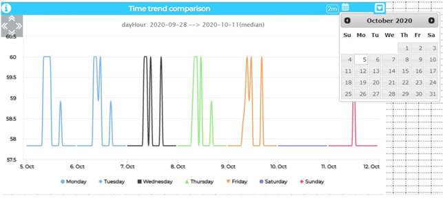
The day hours typical time trend shows 7 different sets of data that refer to the typical trend of the 7 days of the week of the reference period that was requested. In this case then we would have a series of data for each day of the week.
With the calendar at the top right you can change the reference period for which you want to have the typical trend of the sensor.
Month day

The monthDay Typical Time Trend shows the typical trend of the sensor requested, referred to the month requested. The values shown are aligned with the first day of the month.
With the calendar at the top right you can change the reference period for which you want to have the typical trend of the sensor.
Month week
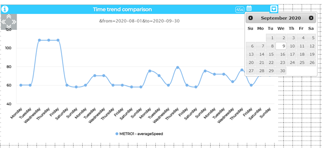
The monthWeek Typical Time Trend shows the typical trend of the requested sensor, referring to the 4 weeks of the requested month. The values shown are aligned to the first Monday of the month.
With the calendar at the top right you can change the reference period for which you want to have the typical trend of the sensor.
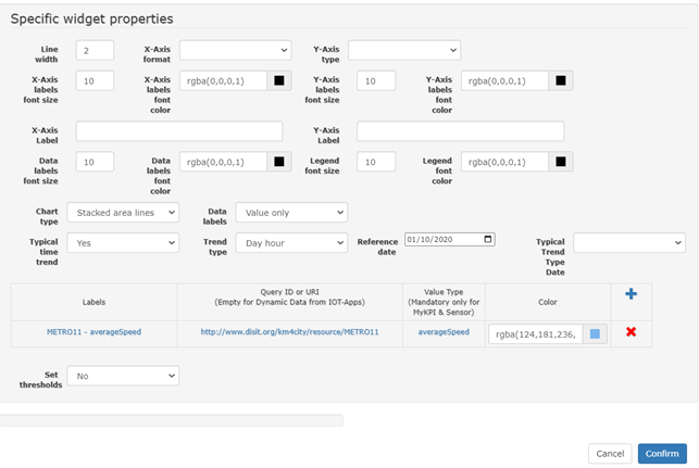
how to set the more options:
In particular,
· The Trend type dropdown menu is available for specific trend types of sensor: Day hours, Month day, Month week.
· The reference date represents the date where to search for typical time trend.
· The typical trend type date vary according to the chosen on Trend Type and on Reference date dropdown menu and shows the interval and the computation type of the typical time trends found through the previous selections.
How to control the production of the Typical Time Trends from R Studio Function
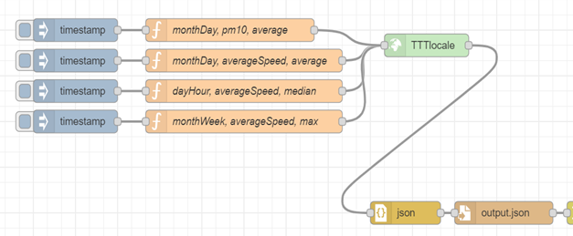
Please note that the block "TTTlocale" is an instance of Plumber RStudio block with loaded the Rstudio function for computing TypicalTimeTrends: https://www.snap4city.org/drupal/sites/default/files/files/ScriptFinal24022021_ips.zip
MonthWeek Input of the RStudio block:
(esempio del trend MonthWeek in riferimento al device METRO11 ed al sensore dell’averageSpeed. Il periodo di interesse è di 2 mesi, la data di riferimento è il 12/10/2020
ed il calcolo si basa sul valore minimo)
{
"serviceUri": "http://www.disit.org/km4city/resource/METRO11/averageSpeed",
"numberOfPeriods": 2,
"referenceDate": "2020-10-12",
"computationType": "min",
"trendType": "monthWeek"
}
MonthWeek Output of the RStudio Block
{ "serviceUri": "http://www.disit.org/km4city/resource/METRO11",
"deviceName": "METRO11",
"valueName": "averageSpeed",
"valueUnit": "km/h",
"referenceDate": "2020-10-12",
"numberOfPeriods": 2,
"from": "2020-08-01",
"to": "2020-09-30",
"trendType": "monthWeek",
"computationType": "min",
"typicalMonthWeek": [ “46.2096”, “51.4195”, “48.7888”, “47.2009”, “36.0467”, “47.6928”, “43.8895”, “47.3346”, “40.8155”, “40.8155”, “44.6956”, “44.6956”, “46.5816”, “43.167”,
“43.8206”, “35.9232”, “47.6799”, “48.1174”, “44.4474”, “44.0122”, “42.9129”, “44.0739”, “47.2921”, “35.1999”, “35.1999”, “46.9519”, “42.8146”, “42.8146”
],
"wrongValues": { "monthWeekError": "No error for this trend" }
}
MonthDay Input:
(esempio del trend MonthDay in riferimento al device METRO11 ed al sensore averageSpeed. Il periodo di interesse è di due mesi, la data di riferimento è il 12/10/2020 ed il tipo di calcolo è la media)
{ "serviceUri": "http://www.disit.org/km4city/resource/METRO11/averageSpeed",
"numberOfPeriods": 2,
"referenceDate": "2020-10-12",
"computationType": "average",
"trendType": "monthDay"
}
MonthDay Output:
{ "serviceUri": "http://www.disit.org/km4city/resource/METRO11",
"deviceName": "METRO11",
"valueName": "averageSpeed",
"valueUnit": "km/h",
"referenceDate": "2020-10-12",
"numberOfPeriods": 2,
"from": "2020-08-01",
"to": "2020-09-30",
"trendType": "monthDay",
"computationType": "average",
"typicalMonthD": [ “59.2039”, “58.8606”, “59.1556”, “59.2643”, “59.2175”, “58.7546”, “59.0367”, “58.89”, “59.0059”, “59.6978”, “59.8696”, “59.5698”, “57.9666”, “59.5293”, “59.3678”, “58.8308”,
“59.8795”, “59.6743”, “59.4784”, “59.1038”, “58.9039”, “58.9305”, “58.7942”, “60.0248”, “59.9674”, “59.9843”, “59.8559”, “59.6011”, “59.486”, “59.4171” ],
"wrongValues": { "monthDayError": "No error for this trend" }
}
DayHour Input:
(esempio del trend DayHour basato sul device METRO11 e sul sensore dell’averageSpeed. Il periodo di calcolo è pari a 2 settimane e la data di riferimento è il 12/10/2020, il calcolo usato è la mediana)
{ "serviceUri": "http://www.disit.org/km4city/resource/METRO11/averageSpeed",
"numberOfPeriods": 2,
"referenceDate": "2020-10-12",
"computationType": "median",
"trendType": "dayHour"
}
DayHour Output:
{ "serviceUri": "http://www.disit.org/km4city/resource/METRO11",
"deviceName": "METRO11",
"valueName": "averageSpeed",
"valueUnit": "km/h",
"referenceDate": "2020-10-12",
"numberOfPeriods": 2,
"from": "2020-09-28",
"to": "2020-10-11",
"trendType": "dayHour",
"computationType": "median",
"typicalDays": { "Monday": [ “60”, “60”, “57.8313”, “57.8313”, “57.8313”, “58.9462”, “59.9926”, “59.0495”, “59.3842”, “59.9658”, “59.9993”, “59.9999”, “60”, “60”, “60”, “60”,
“60”, “60”, “60”, “60”, “60”, “60”, “60”, “60” ],
"Tuesday": [ “58.9157, “57.8313, “57.8313, “57.8313, “57.8313, “58.9767, “59.9976, “59.3196, “59.4856, “59.9507, “59.9985, “59.9999, “60”, “60”, “60”, “60”,
“60”, “60”, “60”, “60”, “60”, “60”, “60”, “60” ],
"Wednesday": [.... ]*, "Thursday": [....]*, "Friday": [......]*, "Saturday": [.....]*, "Sunday": [......]*
},
"wrongValues": { "mondayError": "No error for this trend", "tuesdayError": "No error for this trend",
"wednesdayError": [
"In this period: 2020-09-30T12:00:00 - 2020-09-30T13:00:00 there aren't value",
"In this period: 2020-09-30T13:00:00 - 2020-09-30T14:00:00 there aren't value",
"In this period: 2020-09-30T14:00:00 - 2020-09-30T15:00:00 there aren't value",
"In this period: 2020-09-30T15:00:00 - 2020-09-30T16:00:00 there aren't value",
"In this period: 2020-09-30T16:00:00 - 2020-09-30T17:00:00 there aren't value",
"In this period: 2020-09-30T17:00:00 - 2020-09-30T18:00:00 there aren't value",
"In this period: 2020-09-30T18:00:00 - 2020-09-30T19:00:00 there aren't value",
"In this period: 2020-09-30T19:00:00 - 2020-09-30T20:00:00 there aren't value",
"In this period: 2020-09-30T20:00:00 - 2020-09-30T21:00:00 there aren't value",
"In this period: 2020-09-30T21:00:00 - 2020-09-30T22:00:00 there aren't value",
"In this period: 2020-09-30T22:00:00 - 2020-09-30T23:00:00 there aren't value",
"In this period: 2020-09-30T23:00:00 - 2020-09-30T23:59:59 there aren't value"
],
"thursdayError": [ "In this period: 2020-10-01T00:00:00 - 2020-10-01T01:00:00 there aren't value",
"In this period: 2020-10-01T01:00:00 - 2020-10-01T02:00:00 there aren't value",
"In this period: 2020-10-01T02:00:00 - 2020-10-01T03:00:00 there aren't value",
"In this period: 2020-10-01T03:00:00 - 2020-10-01T04:00:00 there aren't value",
"In this period: 2020-10-01T04:00:00 - 2020-10-01T05:00:00 there aren't value",
"In this period: 2020-10-01T05:00:00 - 2020-10-01T06:00:00 there aren't value",
"In this period: 2020-10-01T06:00:00 - 2020-10-01T07:00:00 there aren't value",
"In this period: 2020-10-01T07:00:00 - 2020-10-01T08:00:00 there aren't value",
"In this period: 2020-10-01T08:00:00 - 2020-10-01T09:00:00 there aren't value",
"In this period: 2020-10-01T09:00:00 - 2020-10-01T10:00:00 there aren't value"
],
"fridayError": "No error for this trend",
"saturdayError": "No error for this trend",
"sundayError": "No error for this trend"
}
}
*Per motivi di spazio, i valori presenti dal mercoledì in poi, sono stati sostituiti da dei puntini.
How to Save the Typical Time Trends

Si noti come debbano essere inseriti tutti i dati necessari alla costruzione del JSON completo, ovvero il JSON che viene prodotto dallo script R presente all’interno del nodo “plumber-data-analytic”. Questi dati vengono combinati e viene costruito il JSON da salvare tramite API.
Nell’IOT app possiamo notare diversi nodi, partendo da sinistra a destra ecco una breve descrizione:
- Inject o Timestamp: Consente l’avvio di tutta la catena presente su node-red;
- Function: Consente l’inserimento dei parametri di input per lo script;
- Plumber-data-analytic, denominato “TTTlocale”: Consente la creazione del servizio che esegue lo script caricato;
- JSON: Effettua la conversione tra String e JSONObject e viceversa;
- File, denominato “output.json”: Preso il JSON dal blocchetto precedente, lo scrive su file, denominato output.json;
- Change: Nodo che effettua un refactor del msg.payload che prima di questo blocchetto era suddiviso in request e response. Dopo questo nodo il risultato dello script passa direttamente tramite msg.payload;
- Save Trends: Blocchetto realizzato durante l’elaborato, di cui se ne parlerà in seguito, che consente il salvataggio dei dati appena prodotti, con gestione di access token incorporata;
- Switch: Consente di indirizzare i risultati dell’elaborazione in 3 dashboard differenti, in base al tipo di trend calcolato;
- Function, denominato “Data Selector”: Funzione che consente di selezionare i dati da inviare, e quindi mostrare, nella dashboard;
- Dashboard, intitolate in base al trend che mostrano: Semplici grafici a linee che mostrano l’andamento dei dati calcolati;
How to retrieve a Typical Time Trend from Storage and API
---work in progress----
---work in progress----
---work in progress----